Modeling Residuals: A Shift in Perspective
In the global linear model, the weather must "compete" with the structure already captured quite effectively by history and the calendar. A substantial portion of its effect is already indirectly accounted for by consumption lags: when it is extremely cold for several days in a row, the high consumption from previous days is already factored into the autoregressive variables. Consequently, the temperature primarily adds redundant or marginal information.This is where the value of adopting a different point of view becomes clear. Instead of trying to learn the total consumption all at once using every input variable, we will break the problem down into two successive steps. First, we keep our baseline model—the one combining the autoregressive history and calendar variables—exactly as it is. This model provides a high-quality initial prediction that captures the bulk of the "average" dynamics: the weekly rhythm, holidays, and the natural inertia of demand.
Once we have this prediction, we calculate the residuals, which are the difference between the actual observed consumption and the consumption predicted by the baseline model:\(\text{residual}(t) = y(t) - \hat{y}_{\text{base}}(t)\)
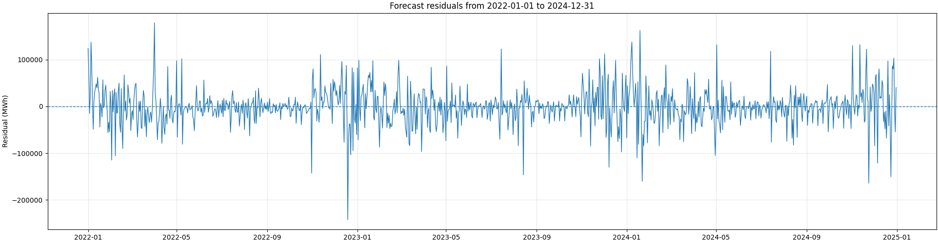
Figure 1 — Displaying residuals for the test period
These residuals, which represent the portion of consumption that the calendar model failed to explain, clearly do not behave like purely random noise. Over the three observed years, their dispersion reveals a recurring temporal structure: it is significantly higher during winter periods, contracts sharply during the summer, and then expands again at the end of the year. This repeated seasonality suggests that a major part of the residual variability is still linked to meteorological factors currently missing from the model—specifically the thermal variables identified during our screening.
Another way to analyze these residuals would be to project them not over time, but within the space of thermal variables, by relating them to an aggregate temperature or heating degree day (HDD) indicators. Such a representation typically highlights the non-linear dependence of consumption on thermal regimes and serves as further motivation to explicitly incorporate meteorological variables.
The idea is therefore to build a second model whose mission is to predict these residuals using meteorological features. Formally, instead of directly learning: \(y(t+1) = f(\text{history, calendar, weather})\)
we proceed in two steps:
\(\hat{y}_{\text{base}}(t+1) = f_{\text{base}}(\text{history, calendar})\)
\(\text{residual}(t+1) = y(t+1) - \hat{y}_{\text{base}}(t+1)\)
\(\hat{y}_{\text{residual}}(t+1) = f_{\text{residual}}(\text{weather, calendar, ...})\)
\(\hat{y}_{\text{final}}(t+1) = \hat{y}_{\text{base}}(t+1) + \hat{y}_{\text{residual}}(t+1)\)
This decomposition offers several notable advantages. First, it considerably simplifies the task for the second model: it no longer has to relearn the entire calendar and temporal structure already well-mastered by the baseline model. It can focus exclusively on the deviations—that is, on situations where the weather truly makes a difference. Second, it makes the approach more modular and robust: the baseline model can be improved or replaced without breaking everything, and vice versa. Finally, it allows for the use of more flexible, non-linear models in the second stage without the risk of them disrupting the stable part of the signal.
We now know exactly what to predict: the residuals of the AR + calendar model. We also know why weather data is a natural candidate for explaining these discrepancies.
However, a major challenge remains: how do we efficiently represent this meteorological information? We have tens of thousands of different ERA5 series at our disposal, corresponding to several thermal variables observed across thousands of geographical coordinates. Feeding all of this data directly into the model would be computationally expensive, unstable, and hard to interpret. Therefore, we must build a more compact representation of the overall thermal state.
The strategy chosen for this tutorial is intentionally simple: instead of searching for "optimal" geographical points, we will summarize the thermal behavior of the entire country using a few aggregated variables. This approach drastically reduces the complexity of the problem while preserving the core meteorological signals needed for the forecast.
This is precisely the objective of the next section.